04.21.2019: One Lesson of Math - Circular Functions, 10/10: Graphing the Trigonometric Reciprocal Fu
- Apr 21, 2019
- 3 min read

Today's soundtrack is Runaway City: Armored Heart, a solid alt-rock album. I don't know why we never heard more from this band; my only guess is that they were a bit too late hopping onto the post-grunge train.
This afternoon, I'm learning how to graph the reciprocal functions.
The reciprocal trigonometric ratios are:
Cosecant
Reciprocal of Sine
Written "csc"
cscθ = (1 / sinθ)
Secant
Reciprocal of Cosine
Written "sec"
secθ = (1 / cosθ)
Cotangent
Reciprocal of Tangent
Written "cot"
cotθ = (1 / tanθ)
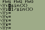
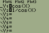
Cosecant and Secant
Much like their reciprocals, sine and cosine, cosecant and secant are very similar to each other. A simple phase shift makes sine and cosine indistinguishable; the same happens with cosecant and secant. I've attached two gifs showing the relationship between these functions and their reciprocals. On the left is sine and cosecant; on the right, cosine and secant.
Reciprocating Sine and Cosine to Produce Cosecant and Secant

To graph the functions of cosecant and secant, we have to recognize what happens to the functions algebraically as we calculate their reciprocal values. If we were to start by graphing a sine or cosine function, we would see a sinusoidal graph with intermittent x-intercepts, repeated maximum y-values of 1, and repeated minimum y-values of -1.
Now if we are to reciprocate each of those features, what happens?
Each x-intercept is located at y 0. If we try to find the reciprocal of 0 by making it the denominator of 1, we'll get an error. So each x-intercept becomes a vertical asymptote.
Next, let's find the reciprocals of the maximums and minimums. Well, 1/1 is still 1, and 1/-1 is still -1. So our maximum and minimum values are invariant points. Finally, we'll find the reciprocals of all the other values. Any very large values will become very small fractions; any small values get larger until they reach our invariant points.
Properties of Cosecant and Secant Functions
Cosecant Properties
Period: 2π
Domain: x ≠ nπ, n∈Z
Range: y ≥ 1, y ≤ -1
Asymptotes: x = nπ, n∈Z
Secant Properties
Period: 2π
Domain: x ≠ π/2+nπ, n∈Z
Range: y ≥ 1, y ≤ -1
Asymptotes: x = π/2+nπ, n∈Z
Transformations of Cosecant and Secant Functions
Our central axis will be the constant at the end of the equation.
To find the minimum and maximum of the graph (the locations of our invariant points), determine the absolute value of the amplitude. Add that value to the value of the central axis to find the maximum; subtract that value from the value of the central axis to find the minimum.
To find the period, calculate 2π/b.
To find the asymptotes (x=) and the domain's restrictions (x≠), first subtract the lowest-value asymptote's value from the next-highest valued asymptote's value. Multiply the difference by n. Next, add the value of the phase shift to n[difference]. This will give the values of the asymptotes and restrictions.
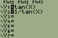
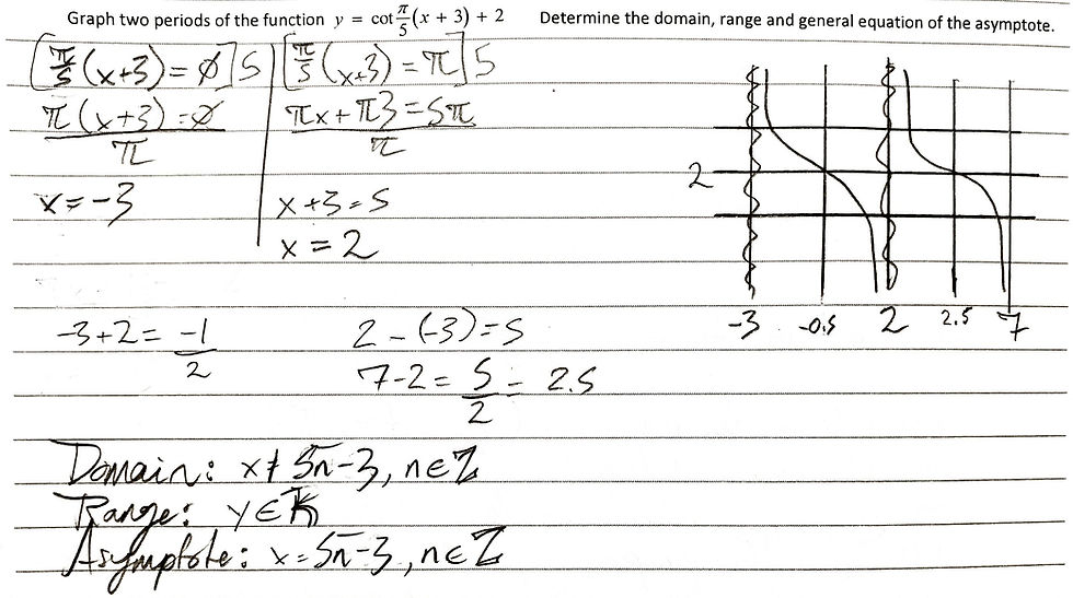
The Cotangent Function
You can see the tangent and the cotangent in their most basic form being graphed in the gif on the left.
The cotangent function looks different from the others, but its essence is the same. It's the reciprocal of the tangent function, and any x-intercepts of the tangent function produce asymptotes. Interestingly, the asymptotes of the tangent function become the x-intercepts of the cotangent.
Properties of the Cotangent Function
Period: π
Domain: x ≠ πn, n∈Z
Range: y∈ℝ
Asymptotes: x = πn, n∈Z
Generating the Cotangent Graph
Rather than graphing the tangent graph and then graphing the cotangent graph over top, we can work out the cotangent graph based on its properties by following these steps:
Find two asymptotes algebraically by solving for x when the argument = nπ, n∈Z.
Determine the distance between the asymptotes by subracting the smaller value from the larger value. The difference is the distance. Use this value to add more asymptotes on if required.
Draw a horizontal line to represent the central axis
Draw the asymptotes as dotted vertical lines, then label
Draw vertical lines between asymptotes
Find the halfway points between the asymptotes by adding their values together and dividing the sum by 2
Mark the central axis with x-intercepts between each asymptote
Mark inflection and infinity points
Halfway between the x-intercept and the asymptote to its left, mark a point of inflection at y1 (or its transformed value), then make a second mark at the top of the graph as close to the left asymptote as you can get.
Halfway between the x-intercept and the asymptote to its right, mark a point of inflection at y -1 (or its transformed value), then make a second mark at the bottom of the graph as close to the right asymptote as you can get.
Draw a smooth line connecting the points.
That's it for today! Next time, I'll be studying for the unit test.
Comments